Calculating a Least Squares Regression Line: Equation, Example, Explanation
If you want a simple explanation of how to calculate and draw a line of best fit through your data, read on!

Complete the form below to unlock access to ALL audio articles.
Being able to make conclusions about data trends is one of the most important steps in both business and science. It’s the bread and butter of the market analyst who realizes Tesla’s stock bombs every time Elon Musk appears on a comedy podcast, as well as the scientist calculating exactly how much rocket fuel is needed to propel a car into space.
Contents
How to find a least squares regression line
Least squares regression line example
Least squares regression equations
How do you calculate a least squares regression line by hand?
How to find a least squares regression line
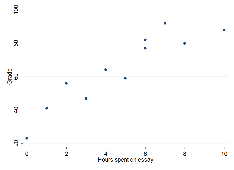
Often the questions we ask require us to make accurate predictions on how one factor affects an outcome. If a teacher is asked to work out how time spent writing an essay affects essay grades, it’s easy to look at a graph of time spent writing essays and essay grades say “Hey, people who spend more time on their essays are getting better grades.” What is much harder (and realistically, pretty impossible) to do by eye is to try and predict what score someone will get in an essay based on how long they spent on it. Sure, there are other factors at play like how good the student is at that particular class, but we’re going to ignore confounding factors like this for now and work through a simple example.
Our teacher already knows there is a positive relationship between how much time was spent on an essay and the grade the essay gets, but we’re going to need some data to demonstrate this properly.
Least squares regression line example

Least squares regression equations


How do you calculate a least squares regression line by hand?
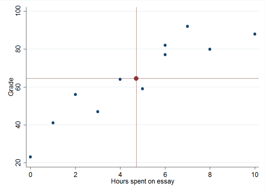
The second step is to calculate the difference between each value and the mean value for both the dependent and the independent variable. In this case this means we subtract 64.45 from each test score and 4.72 from each time data point. Additionally, we want to find the product of multiplying these two differences together.

You should notice that as some scores are lower than the mean score, we end up with negative values. By squaring these differences, we end up with a standardized measure of deviation from the mean regardless of whether the values are more or less than the mean.
Let's remind ourselves of the equation we need to calculate b.
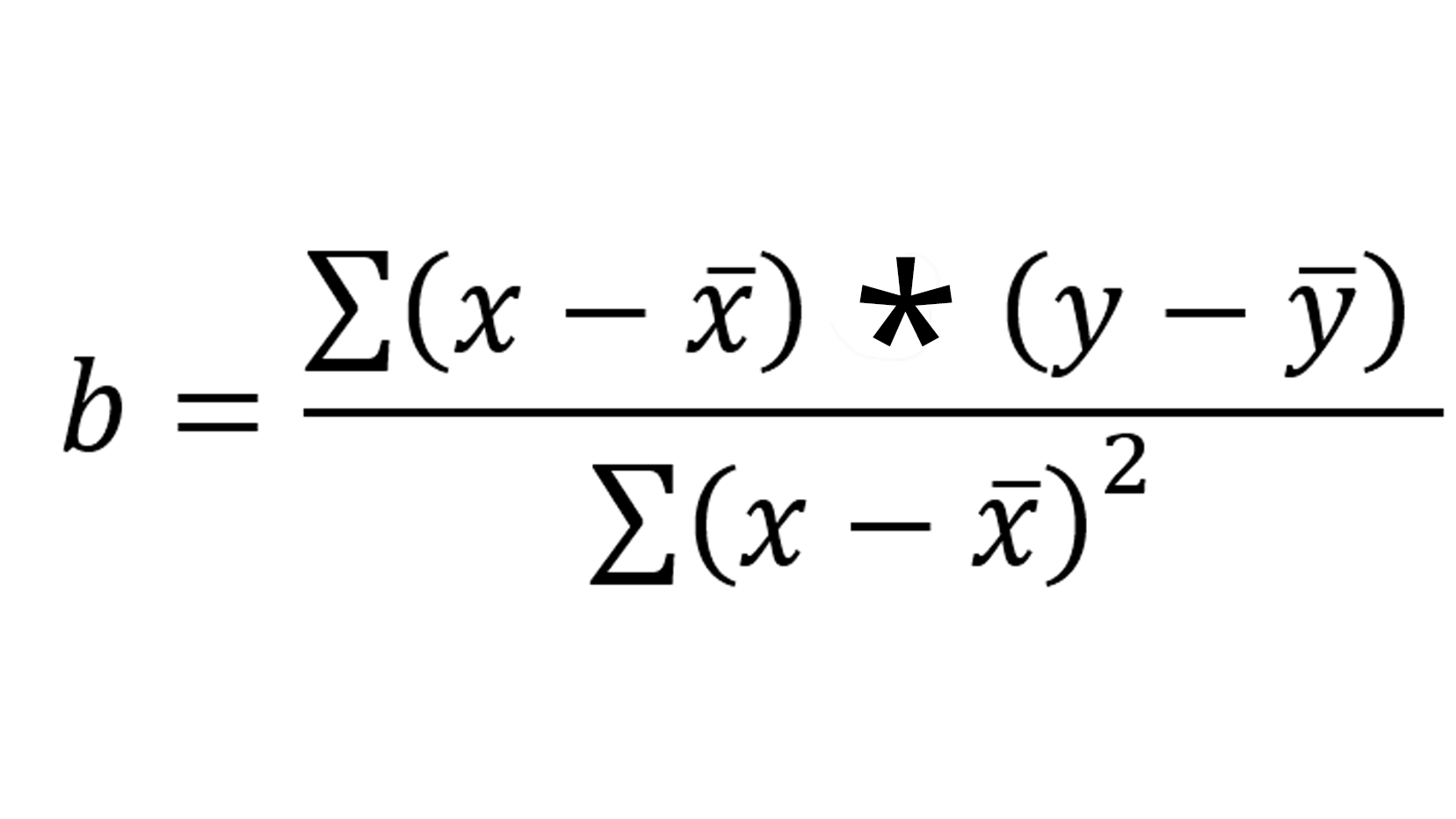
The symbol sigma (∑) tells us we need to add all the relevant values together.
If we do this for the table above, we get the following results:
∑(x-x ̅ ) * (y-y ̅ ) = 611.36
And
∑(x-x ̅ ) ^2 = 94.18
Slotting in the information from the above table into a calculator allows us to calculate b, which is step one of two to unlock the predictive power of our shiny new model:

The final step is to calculate the intercept, which we can do using the initial regression equation with the values of test score and time spent set as their respective means, along with our newly calculated coefficient.
64.45= a + 6.49*4.72
We can then solve this for a:
64.45 = a + 30.63
a = 64.45 – 30.63
a = 30.18
Now we have all the information needed for our equation and are free to slot in values as we see fit. If we wanted to know the predicted grade of someone who spends 2.35 hours on their essay, all we need to do is swap that in for X.
y=30.18 + 6.49 * X
y = 30.18 + (6.49 * 2.35)
y = 45.43
Drawing a least squares regression line by hand
If we wanted to draw a line of best fit, we could calculate the estimated grade for a series of time values and then connect them with a ruler. As we mentioned before, this line should cross the means of both the time spent on the essay and the mean grade received.
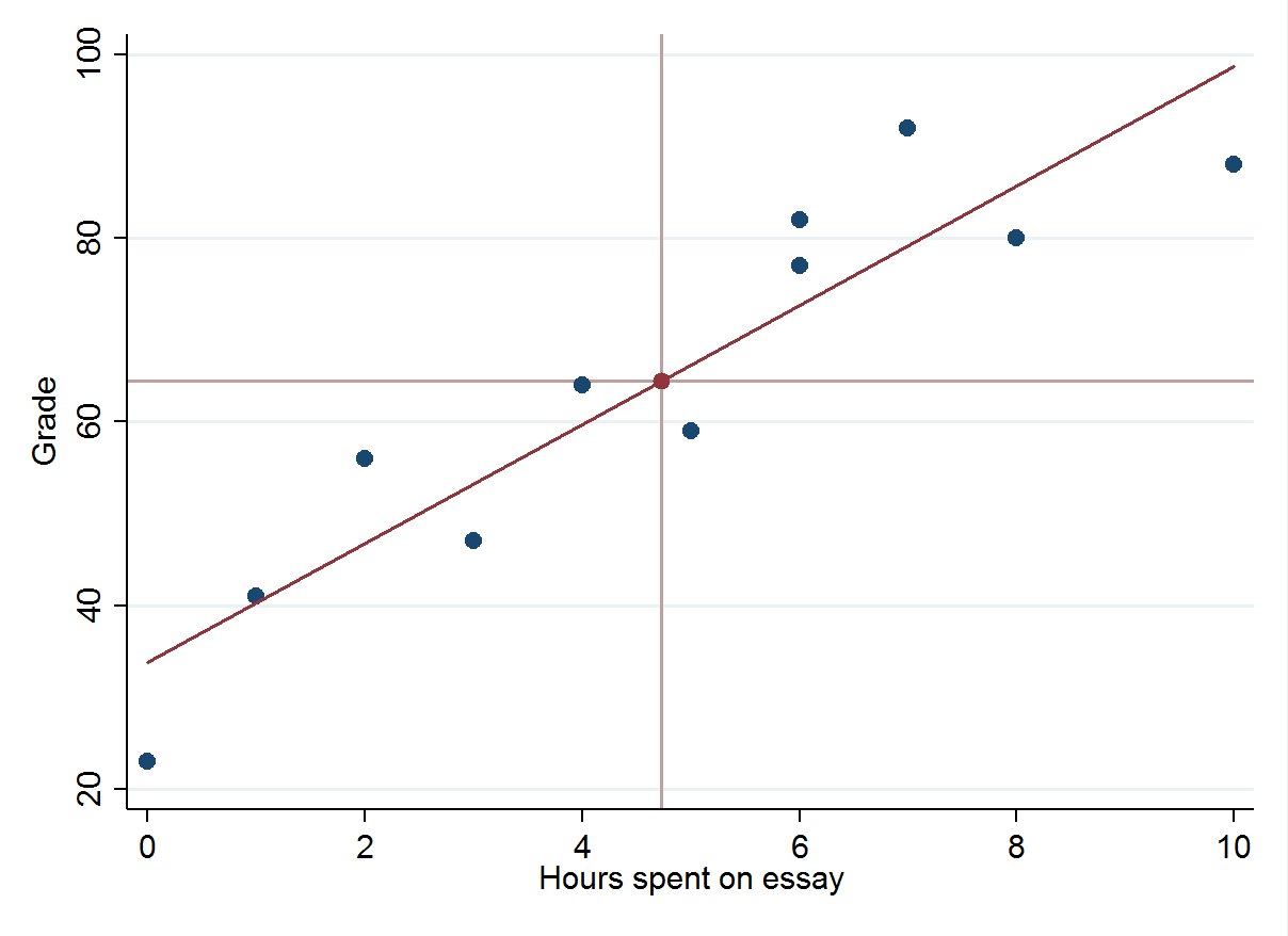
And there we have it! A perfect* predictive model that will make our teachers’ lives a lot easier.
What are the disadvantages of least-squares regression?
*As some of you will have noticed, a model such as this has its limitations. For example, if a student had spent 20 hours on an essay, their predicted score would be 160, which doesn’t really make sense on a typical 0-100 scale. It’s always important to understand the realistic real-world limitations of a model and ensure that it’s not being used to answer questions that it’s not suited for. 
Outliers such as these can have a disproportionate effect on our data. In this case, it's important to organize your data and validate your model depending on what your data looks like to make sure it is the right approach to take.